PRIVATE ONE-ON-ONE TUITION · ONLINE WORLDWIDE

Why Does a Ramsey Economy Ride Its Saddle Path? A Boston Macroeconomics Tutor’s Walkthrough of Ramsey–Cass–Koopmans for Harvard and MIT

Microeconomics · Macroeconomics · Econometrics & Finance

In 1928 Frank Ramsey asked how much of its income a nation ought to save, and answered with a differential equation. In 1965 David Cass and Tjalling Koopmans, working separately, set his question on top of the neoclassical growth model, and the result became a workhorse of modern macroeconomics. If first-year graduate macro at Harvard or MIT, or an advanced macro course at Boston University, Boston College, Tufts or Northeastern, has just handed you a Hamiltonian and a phase diagram, this is the Ramsey–Cass–Koopmans lesson a Boston macroeconomics tutor would give you. You get the model in full, the saddle path derived rather than sketched, and one economy solved exactly, from its eigenvalues to its first-period consumption.

What Solow left out: a saving rate that chooses itself

In the Solow growth model, households save a fixed share s of output. That keeps the dynamics one-dimensional and the steady state easy to find. It also leaves the model silent on the question you most want answered: is that saving rate any good? A high enough s pushes capital past the golden rule, where everyone could consume more forever by saving less. Nothing in Solow prevents it.

Ramsey–Cass–Koopmans swaps the fixed s for a decision. Households trade consumption today against consumption later, and the return they earn is the marginal product of the capital they collectively own, net of depreciation. Two results follow. Saving now responds to the state of the economy, so in general it changes along the transition. And the steady state can never sit above the golden rule, which this page proves. The price of those results is a second dynamic variable. Consumption joins capital, and a single differential equation becomes a two-dimensional system with a saddle point. Add shocks to technology and a labour–leisure choice, and the same machinery becomes the core of real business cycle theory.

The planner’s problem in effective units

Output is Y = F(K, AL) with constant returns, so per effective worker y = f(k), where k = K/(AL), f(0) = 0, f′ > 0, f″ < 0 and the Inada conditions hold. The labour force L grows at rate n, technology A at rate g, and capital depreciates at rate δ. Labour is supplied inelastically.

There are H identical dynastic households, each with L/H members. Write C for consumption per person. Each household maximises

$U = \int_0^\infty e^{-\rho t}\,\frac{C(t)^{1-\theta}}{1-\theta}\,\frac{L(t)}{H}\,dt, \qquad \theta > 0$

so ρ is the rate of time preference and 1/θ is the intertemporal elasticity of substitution. At θ = 1 read the utility term as ln C. Now let c = C/A, consumption per person in efficiency units. Since everyone works, C/A is also total consumption divided by AL, so c is consumption per effective worker, the same unit as k. Substituting C = Ac and the growth paths of A and L turns the objective into

$U = B\int_0^\infty e^{-\beta t}\,\frac{c(t)^{1-\theta}}{1-\theta}\,dt, \qquad \beta \equiv \rho - n - (1-\theta)\,g$

where B = A(0)^1−θL(0)/H is a positive constant. Assume β > 0. Otherwise the integral diverges along feasible paths and no path can be ranked against another. Output per effective worker is split between consumption and investment, which gives the resource constraint

$\dot k = f(k) - c - (n+g+\delta)\,k, \qquad k(0) \text{ given}$

The decentralised version has competitive firms paying a rental rate f′(k), so the net return on capital is r = f′(k) − δ, and a wage per effective worker of f(k) − kf′(k). Households are price-takers who own the capital, supply their labour and face a no-Ponzi condition on their debt. With complete markets and no externalities or distortions, the first welfare theorem makes the competitive path the planner’s path. Solve whichever is quicker. Here that is the planner.

Deriving the Keynes–Ramsey rule

Use the current-value Hamiltonian, with μ the shadow value of a unit of capital per effective worker.

$\mathcal{H}(k,c,\mu) = \frac{c^{1-\theta}}{1-\theta} + \mu\,\big[f(k) - c - (n+g+\delta)\,k\big]$

The maximum principle gives two conditions. Consumption is chosen so that its marginal utility equals the shadow value of capital, and the shadow value evolves like the price of an asset.

$c^{-\theta} = \mu, \qquad\qquad \dot\mu = \beta\mu - \frac{\partial \mathcal{H}}{\partial k} = \mu\,\big[\beta + n + g + \delta - f'(k)\big]$

Log-differentiate the first condition: −θ ċ/c = μ̇/μ. Substitute the second and expand β. The n terms cancel, and so does one g.

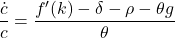
$\frac{\dot c}{c} = \frac{f'(k) - \delta - \rho - \theta g}{\theta}$

That is the Keynes–Ramsey rule. Rewritten for consumption per person it reads Ċ/C = (r − ρ)/θ. Consumption grows when the return on capital beats impatience, and the more willing households are to shift consumption across time, the more strongly it responds to that gap. If the two-period version is rusty, the Euler equation for consumption smoothing is the same trade-off with one period of waiting instead of a continuum.

An infinite horizon also needs a terminal condition, the transversality condition. In this concave problem with β > 0 it is necessary, and together with the Euler equation it is sufficient for an optimum.

$\lim_{t\to\infty} e^{-\beta t}\,\mu(t)\,k(t) = 0 \quad\Longleftrightarrow\quad \lim_{t\to\infty} k(t)\,\exp\Big(-\int_0^t \big[r(s) - n - g\big]\,ds\Big) = 0$

In words, the present value of the capital left over at the end of time must be zero. The Euler equation and the resource constraint are two differential equations, and you have only one initial condition, k(0). Transversality, together with the requirement that capital never go negative, supplies the missing boundary condition. Between them they pin down c(0).

Reading the phase diagram

Draw the system in (k, c) space. Each equation contributes one locus.

ċ = 0 where f′(k) = ρ + δ + θg. Because f′ is decreasing, this is a vertical line at a single k*. To its left f′ is higher, so consumption rises. To its right it falls.
k̇ = 0 where c = f(k) − (n + g + δ)k. This locus is a hump. It peaks where f′(k) = n + g + δ, the golden rule, and meets the axis again at a maximum sustainable capital stock k̄. Above the hump, consumption eats into capital and k falls. Below it, k rises.

With c > 0 the loci cross once, at the steady state. (The axis c = 0 is a trivial ċ = 0 locus, so the origin and (k̄, 0) are also rest points.)

$f'(k^*) = \rho + \delta + \theta g, \qquad c^* = f(k^*) - (n+g+\delta)\,k^*$

This is the modified golden rule. Since β > 0 means ρ + θg > n + g, the steady-state marginal product exceeds n + g + δ, and so k* lies to the left of the golden-rule capital stock k_GR. The steady state never over-accumulates. The reason is the effective discount rate β = (ρ − n) + (θ − 1)g, which combines impatience net of population growth with the wish to smooth consumption when later generations will be richer. Lifting steady-state consumption all the way to the golden rule would cost a sacrifice now that this discounting says is not worth making.

Figure 1. The phase diagram for f(k) = k^1/3, δ = 0.05, n = 0.01, g = 0.02, ρ = 0.02 and θ = 2. The saddle path is computed exactly from the nonlinear system. From A, at half the steady-state capital stock, only c(0) = 0.973 leads to E. The dashed paths start 0.12 above and 0.12 below it. GR marks the golden rule.

Now fix k(0) at point A and ask which c(0) the household should pick. Start too high, on the upper dashed path. Consumption climbs throughout, while capital edges up and then drains away. In this calibration it hits zero within about 11 years. At that moment output is zero, so consumption would have to drop to zero in an instant, and the Euler equation forbids a jump in consumption at a date everyone saw coming. No continuation of that path is both feasible and consistent with the Euler equation, so it is not an optimum.

Start too low, on the lower dashed path. Capital overshoots k*, consumption peaks and then slides toward zero, and the economy creeps toward the rest point (k̄, 0), with k̄ about 44.2 here. Once k passes the golden rule, r falls below n + g. The exponential term in the transversality condition then grows instead of shrinking while k stays large, so the condition fails. The household is piling up capital it will never consume. Eating some of it would be feasible and would raise utility, so this path is not an optimum either.

Exactly one choice of c(0) lands on the stable arm and converges to E. That arm is the saddle path, and it defines consumption as a function of capital, c(k), at every date.

Linearising around the steady state

Near E, replace the system by its first-order Taylor expansion.

$\begin{pmatrix}\dot k\\ \dot c\end{pmatrix} \approx \begin{pmatrix} \beta & -1\\ c^*f''(k^*)/\theta & 0\end{pmatrix}\begin{pmatrix}k - k^*\\ c - c^*\end{pmatrix}$

Two entries deserve a line each. The top-left is f′(k*) − (n + g + δ) = ρ + θg − n − g, which is exactly β. The bottom-right is zero because the bracket in the Keynes–Ramsey rule vanishes at k*, so a small change in c alone does not move ċ.

The determinant is c*f″(k*)/θ, which is negative. A negative determinant means two real eigenvalues of opposite sign: a saddle. The trace is β, so

$\lambda_{1,2} = \frac{\beta \mp \sqrt{\beta^2 - 4c^*f''(k^*)/\theta}}{2}, \qquad \lambda_1 < 0 < \lambda_2$

Along the stable arm only λ₁ operates. The first row of the system says the eigenvector satisfies (β − λ₁)·(k − k*) = c − c*. And because λ₁ + λ₂ = β, the slope β − λ₁ is simply λ₂.

$k(t) - k^* = e^{\lambda_1 t}\,\big(k(0) - k^*\big), \qquad c(t) - c^* = \lambda_2\,\big(k(t) - k^*\big)$

The counting is worth stating out loud. There is one predetermined variable, k, and one jump variable, c. There is one unstable root. That match is the continuous-time analogue of the Blanchard–Kahn condition (Blanchard and Kahn, 1980, Econometrica), and it makes the solution of the linearised system unique. The phase-diagram argument above gives the global result. Capital closes its gap to k* at the continuous rate |λ₁|, so the half-life of the gap is ln 2/|λ₁|.

One economy, rebuilt from half its capital

Take an economy whose capital stock has been halved, say by a war that left its workers and its technology intact. Production is Cobb–Douglas, f(k) = k^1/3, and the annual parameters are those in Figure 1: δ = 0.05, n = 0.01, g = 0.02, ρ = 0.02 and θ = 2.

The discount condition. β = 0.02 − 0.01 − (1 − 2)(0.02) = 0.03. It is positive, so lifetime utility is finite.
The steady state. f′(k*) = 0.02 + 0.05 + 2 × 0.02 = 0.11. With f′(k) = ⅓k^−2/3, that gives k* = 5.275. Output is y* = 1.741, and consumption is c* = 1.741 − 0.08 × 5.275 = 1.319.
The saving rate. Gross investment (n + g + δ)k* as a share of output is s* = α(n + g + δ)/(ρ + δ + θg) = ⅓ × 0.08/0.11 = 24.2%. Here α = ⅓ is the capital exponent, and the closed form holds for any Cobb–Douglas economy.
The golden rule. Setting f′(k) = 0.08 gives k_GR = 8.505 and c_GR = 1.361. The steady state holds 38% less capital than the golden rule. That gap is the effective discount rate at work.
Transversality. r* = 0.11 − 0.05 = 6%, above n + g = 3%. The margin is 3 points, which is β again. At the steady state the two conditions are one condition.
The Jacobian. f″(k*) = (α − 1)f′(k*)/k* = −0.0139, so the bottom-left entry is 1.319 × (−0.0139)/2 = −0.00917. The discriminant is 0.03² + 4 × 0.00917 = 0.0376, whose square root is 0.1938.
The eigenvalues. λ₁ = (0.03 − 0.1938)/2 = −0.0819 and λ₂ = (0.03 + 0.1938)/2 = 0.1119. The stable arm has slope 0.1119 at E, and the half-life of the capital gap is ln 2/0.0819 = 8.46 years.
Consumption on day one. k(0) = 5.275/2 = 2.638. The linear rule gives c(0) ≈ 1.319 + 0.1119 × (2.638 − 5.275) = 1.024. Integrating the nonlinear system backwards from E gives the exact saddle path, and on it c(0) = 0.973. The linear rule overstates first-period consumption by about 5%. It also understates the time needed: the exact path takes 8.94 years to close half the gap, not 8.46.
Prices and saving along the way. At A the scarce capital earns r(0) = f′(2.638) − 0.05 = 12.5%, and consumption per effective worker grows at 3.2% a year. The saving rate is 1 − 0.973/2.638^1/3 = 29.6%. It then falls steadily to 24.2% as the economy approaches E.

Step 9 is the result Solow cannot produce. Two forces pull on saving when capital is scarce. The high return invites you to save more, which is substitution. The knowledge that you will be richer later invites you to consume more now, which is the income effect. With Cobb–Douglas production the contest has a clean verdict. Starting below k*, the saving rate falls along the path when s* < 1/θ, stays constant when s* = 1/θ, and rises when s* > 1/θ. Here 0.242 is well below 0.5, so it falls. Keep every other number and set θ = 10.5: then s* = 0.0952 = 1/θ exactly, and the saving rate is flat along the whole saddle path.

A surprise rise in patience

Now suppose the economy is resting at E when households unexpectedly and permanently become more patient: ρ falls from 0.02 to 0.01.

Figure 2. An unanticipated, permanent fall in ρ from 0.02 to 0.01. Capital cannot jump, so consumption drops from E straight down to J on the new saddle path. Consumption and capital then rise together to E′.

The k̇ = 0 locus does not contain ρ, so it stays where it is. The ċ = 0 line moves right, to where f′(k) = 0.01 + 0.05 + 0.04 = 0.10. The new steady state E′ has k*′ = 6.086, c*′ = 1.339 and a saving rate of 26.7%.

Capital at the moment of the news is 5.275, and capital is a stock. It cannot move until investment moves it. Consumption is the only thing free to adjust, and it must jump to the one value that puts the economy on the new saddle path. That value is 1.258, a fall of 0.061, or 4.6% of the old c*. The saving rate jumps from 24.2% to 27.7% on impact. From J, capital accumulates and consumption rises with it toward E′, more slowly than the old economy would have, since the new stable root is −0.0762 against the old −0.0819.

The long run rewards the sacrifice. Steady-state consumption ends at 1.339, above the old 1.319, because k*′ is still below the golden rule of 8.505. More patience means less consumption now and more later.

Where problem-set answers slip

A common algebra error is dropping the θg term. In effective units the ċ = 0 line is f′(k) = ρ + δ + θg, not ρ + δ. In the worked example that term is 4 points of return. Leave it out and you set f′(k) = 0.07, which gives k = 10.39. That is above the golden rule, and a Ramsey steady state above the golden rule should itself have set off an alarm.

Next comes letting capital jump. After an unanticipated change in a parameter such as ρ, n, δ or G, k stays put and c does all the jumping. If your phase diagram shows the economy sliding horizontally to a new saddle path, the diagram is wrong. Anticipated changes in such parameters are subtler. Consumption jumps once, at the announcement. Between the announcement and the date the change takes effect, the economy follows the old equations, and it must arrive on the new saddle path exactly when the change bites. A second jump on a known date would mean a predictable jump in marginal utility, which the Euler equation rules out.

Third, transversality is often cited and never used. Say which paths it eliminates. It kills the paths on which consumption starts too low and capital heads toward k̄. Paths on which consumption starts too high fail for a different reason: they run capital to zero, after which no continuation is both feasible and consistent with the Euler equation.

Fourth, students often confuse the two golden rules and then claim the economy might be dynamically inefficient. It cannot be. The competitive path solves the planner’s problem, the steady state sits below the golden rule whenever β > 0, and transversality keeps r above n + g in the long run. Dynamic inefficiency is possible in Diamond’s (1965) overlapping-generations model, where finitely lived generations with no operative bequest motive follow one another forever.

Finally, check whether a linearised answer has been passed off as exact. The linear rule is a statement about a neighbourhood of E. At half the steady-state capital stock it already overstates c(0) by 5% in the example above. If a question asks for the speed of convergence, say that both the speed |λ₁| and the half-life ln 2/|λ₁| describe behaviour near E.

If you are meeting this model in the first-year macro sequence at Harvard or MIT, or in advanced macro at BU, BC, Tufts or Northeastern, the Hamiltonian is usually not where marks are lost. They tend to go at the boundary conditions, the jump variables and the linearisation. Good macroeconomics tutoring for Harvard and MIT students works on exactly those, using your own problem-set calibration: solve it the way this page does, then find where your phase diagram and your algebra disagree. See how a session works.

Three problems to work, with answers

Problem 1 (warm-up). Let f(k) = k^1/2, δ = 0.06, n = 0.01, g = 0.01, ρ = 0.03 and θ = 1, which is the log-utility limit of the CRRA form. Check the discount condition. Find k*, y*, c*, the saving rate s* and the golden-rule capital stock, then confirm that transversality holds at the steady state.

Answer. β = 0.03 − 0.01 − 0 = 0.02 > 0. The steady state needs f′(k*) = 0.03 + 0.06 + 0.01 = 0.10, so ½k^−1/2 = 0.10 and k* = 25. Then y* = 5 and c* = 5 − 0.08 × 25 = 3, so s* = 2/5 = 40%. The golden rule needs ½k^−1/2 = 0.08, so k_GR = 39.06, well above k*. Finally r* = 0.10 − 0.06 = 4%, above n + g = 2%.

Problem 2 (fiscal policy). In the economy of the worked example, the government starts buying G = 0.1 per effective worker, permanently and without warning, financed by lump-sum taxes. G is constant per effective worker and enters neither utility nor production. The resource constraint becomes k̇ = f(k) − c − G − (n + g + δ)k. What happens to k and c on impact and in the long run?

Answer. The k̇ = 0 locus shifts down by 0.1 at every k. The Keynes–Ramsey rule does not contain G, so the ċ = 0 line stays at k* = 5.275. The new steady state therefore has the same capital and consumption 1.319 − 0.1 = 1.219. Capital does not need to move, so the economy jumps straight to the new steady state: consumption falls by exactly 0.1 on impact, and there is no transition at all. An unanticipated temporary purchase is different. Consumption falls by less than G, and capital absorbs part of the cost while the purchase lasts.

Problem 3 (hard: the transition). Use Problem 1’s economy, but start it at k(0) = 16. Find the Jacobian at the steady state, both eigenvalues, the slope of the saddle path at E, the half-life of the capital gap and the linear approximation to c(0). The exact saddle path gives c(0) = 2.167. Which way is the linear rule wrong, what saving rate does the exact value imply, and does saving rise or fall from there?

Answer. f″(25) = −½ × 0.10/25 = −0.002, so the bottom-left entry is 3 × (−0.002)/1 = −0.006. The top-left entry is β = 0.02. The eigenvalues are (0.02 ∓ √(0.0004 + 0.024))/2, that is λ₁ = −0.0681 and λ₂ = 0.0881. The saddle path’s slope at E is 0.0881, and the half-life is ln 2/0.0681 = 10.18 years. The linear rule gives c(0) ≈ 3 + 0.0881 × (16 − 25) = 2.207, which overstates the exact 2.167 by 0.04, the same direction as in the worked example. Output at k = 16 is 4, so the exact saving rate is 1 − 2.167/4 = 45.8%. Since s* = 0.4 is below 1/θ = 1, saving falls along the path toward 40%.

Book a Boston macroeconomics tutor for the growth half of first-year macro

Growth theory tends to arrive midway through a first-year sequence, just as the problem sets get longer. Send the calibration that will not converge or the phase diagram that will not close, and you will be matched with a PhD tutor who works comfortably in continuous time. Sessions run online, so a macro tutor in Boston fits around your section times. Request a first session, or message from the WhatsApp button at the top of the page.

Get Started