
When unemployment rises by a point, how much output has the economy given up? Okun’s law answers that with one number, and intermediate macro leans on it constantly: to size a recession, to translate a Phillips curve into lost GDP, to read a Taylor rule. This Okun’s law lesson, written by a Washington DC macroeconomics tutor, builds the relationship from the ground up. You get both forms, the derivation that links them, the reason the coefficient is about two rather than one, and a worked path you can check line by line.
Two numbers that move together
Unemployment and output are not independent facts about an economy. When firms produce less, they need fewer workers, and some of the people they let go cannot find other jobs. So the unemployment rate climbs when output falls short of what the economy could produce, and it falls when output runs ahead.
Arthur Okun put a number on this in 1962, in a paper for the American Statistical Association on measuring potential GNP. His estimate for postwar US data was that each percentage point of unemployment above its normal level went with roughly three percent less output. The relationship is empirical. It is not derived from a model of firms or households, and that matters later: its coefficient is a summary of several behaviours at once, and it can change when those behaviours change.
The word that does the work is potential. Potential output, Y*, is what the economy produces when unemployment sits at its natural rate, u*, the rate consistent with stable inflation. Neither is observed. Both are estimated, and in the United States most courses use the potential-output series the Congressional Budget Office publishes. The output gap is the percentage distance between actual and potential output, the same gap that drives the short-run equilibrium in the AD–AS model.
The gap form
The cleanest statement of Okun’s law ties the two gaps together:
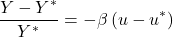
The left side is the output gap in percent. The right side is the unemployment gap in percentage points, scaled by the Okun coefficient β. With β = 2, unemployment one point above the natural rate means output two percent below potential. The minus sign carries the direction: a negative output gap goes with unemployment above its natural rate.
Read it in both directions. Given an unemployment rate, it tells you the output gap. Given a forecast of the output gap, it tells you where unemployment is heading. That second use is how forecasters translate a GDP projection into a jobs projection.
From levels to growth rates
Most data arrive as growth rates, not gaps, so you need the second form. Work in logs, because a log difference is a percentage change. Define the output gap as

Now difference it from one year to the next:

The change in the gap is actual growth g minus potential growth g*. Apply the gap form in year t and year t − 1 and subtract. If the natural rate is constant, the u* terms cancel:

This is the difference form. It says something students often find surprising. Unemployment does not fall just because the economy grows. It falls only when the economy grows faster than potential. Growth exactly at potential leaves unemployment where it was, and growth that is positive but below potential pushes it up.
Two cautions. The step from the gap form to the difference form assumed u* fixed. If the natural rate drifts, Δu* appears on the right and the clean line shifts. And the log approximation is good for gaps of a few percent. It loosens in deep recessions, though not enough to change any conclusion at intermediate level.
Why the coefficient is about two, not one
Suppose every worker produced the same amount and worked the same hours. Then a one-point rise in unemployment would remove one percent of the labour force from production, and output would fall by about one percent. β would be one. Okun found about three; modern US estimates are closer to two. Where does the extra come from?
Split output into four factors. Let H be total hours, E employment and L the labour force:

Taking logs turns the product into a sum, and ln(1 − u) ≈ −u, so the employment-rate term moves one-for-one with unemployment. The other three terms are what push β above one. Output per hour has historically fallen in downturns, because firms keep skilled staff on through a slump rather than lose them: labour hoarding. (The pattern has weakened in recent US recessions.) Hours per worker fall as overtime disappears and part-time work grows. And the labour force itself shrinks relative to trend, as discouraged workers stop searching and are no longer counted as unemployed.
Here is a downturn in which output ends up 2 percent below trend. In log points relative to trend:
| Margin | Change |
|---|---|
| Output per hour, Y/H | −0.6 |
| Hours per worker, H/E | −0.3 |
| Employment rate, E/L | −1.0 |
| Labour force, L | −0.1 |
| Output, Y | −2.0 |
Unemployment rose by one point, which is the −1.0 on the employment-rate line. Output fell by 2.0. The ratio, 2, is the Okun coefficient. Only half of the output loss shows up as unemployment, and the rest is absorbed by productivity, hours and participation. That is why the law is a regularity rather than an identity: change how firms hoard labour or how workers respond to slack, and β changes too. Ball, Leigh and Loungani (2017, Journal of Money, Credit and Banking) find the relationship strong and fairly stable within most advanced economies, with coefficients that differ considerably from one country to another.
Four years, worked through
Take an economy with potential growth g* = 2.5 percent, an Okun coefficient β = 2 and a natural rate u* = 4.5 percent. In year 0 it sits at potential, so unemployment is 4.5 percent and the output gap is zero. Then growth comes in at 1.0, −0.5, 2.5 and 4.5 percent over the next four years.
Step 1 is the difference form, year by year. In year 1, growth falls short of potential by 1.5 points, so Δu = −(1.0 − 2.5)/2 = +0.75. Step 2 accumulates the changes into a level. Step 3 builds the output gap from the growth shortfalls, and step 4 cross-checks it against the gap form, −2(u − 4.5).
| Year | Growth g (%) | Δu (points) | u (%) | Output gap (%) |
|---|---|---|---|---|
| 0 | — | — | 4.5 | 0 |
| 1 | 1.0 | +0.75 | 5.25 | −1.5 |
| 2 | −0.5 | +1.5 | 6.75 | −4.5 |
| 3 | 2.5 | 0 | 6.75 | −4.5 |
| 4 | 4.5 | −1.0 | 5.75 | −2.5 |
Both routes to the output gap agree in every year. In year 2, for example, the growth shortfalls add up to −1.5 − 3.0 = −4.5, and the gap form gives −2 × (6.75 − 4.5) = −4.5.
Step 5 is reading the table, and three lessons come out of it. Year 1 has positive growth and rising unemployment, the pattern sometimes called a growth recession. Year 3 is the subtle one. The economy has returned to its normal growth rate, which feels like recovery, yet unemployment is stuck at 6.75 percent and the gap has not closed at all, because growth at potential only holds the gap where it is. Closing it requires a stretch of above-potential growth, which year 4 begins.
Step 6 asks how fast the economy would have to grow in year 5 to bring unemployment back to 4.5 percent in a single year. Unemployment must fall by 1.25 points, so growth must exceed potential by 2 × 1.25 = 2.5 points: 5.0 percent. Step 7 adds up the damage. Summing the four gaps gives −13, so over the episode the economy lost output equal to 13 percent of one year’s potential. That figure is the cost of the recession, and it is far larger than any single year suggests.
Where Okun’s law meets the Phillips curve
The law earns its place in the syllabus by connecting the labour market to everything measured in output. The clearest example is the cost of disinflation. An expectations-augmented Phillips curve, πt = πt−1 − α(ut − u*), says inflation falls only while unemployment sits above its natural rate. With α = 0.5, cutting inflation by 2 points needs 2/0.5 = 4 point-years of excess unemployment, however you spread them in this backward-looking model.
Okun’s law converts that into output. With β = 2, four point-years of excess unemployment cost 2 × 4 = 8 percent of a year’s GDP. Divide by the 2 points of disinflation and you have the sacrifice ratio in output terms: 4 percent of GDP per point of inflation removed. A central bank weighing a tighter path, for instance one implied by a Taylor rule, is weighing exactly this number. Notice what drives it: a flat Phillips curve (small α) or a large Okun coefficient both make disinflation expensive.
Problems to try
Problem 1. Potential growth is 2 percent and β = 2. Real GDP grows 0.5 percent this year and the natural rate does not change. What happens to the unemployment rate?
Answer. Δu = −(0.5 − 2)/2 = +0.75. Unemployment rises by three-quarters of a point despite positive growth.
Problem 2. The natural rate is 4 percent, actual unemployment is 6.5 percent and β = 2. Potential output is 25 trillion USD. Find the output gap and the output lost this year.
Answer. The unemployment gap is 2.5 points, so the output gap is −2 × 2.5 = −5 percent. Output is 5 percent of 25 trillion below potential, a shortfall of 1.25 trillion USD.
Problem 3. A central bank wants to bring inflation down by 3 points. The Phillips curve slope is α = 0.4 and the Okun coefficient is β = 2.5. Find the excess unemployment required in point-years, the total output cost and the sacrifice ratio. If the disinflation is spread evenly over three years, what are the unemployment gap and the output gap in each year?
Answer. Point-years of excess unemployment: 3/0.4 = 7.5. Output cost: 2.5 × 7.5 = 18.75 percent of a year’s GDP. Sacrifice ratio: 18.75/3 = 6.25. Spread evenly, unemployment sits 2.5 points above the natural rate in each year, and the output gap is −2.5 × 2.5 = −6.25 percent each year. In this model, with adaptive expectations, the cost depends only on the total, not the timing. If policy is credible and expectations adjust faster, the cost can be lower.
A macroeconomics tutor for Georgetown, GW, Johns Hopkins and Maryland students
If your intermediate macro course at Georgetown, George Washington University, American University, Johns Hopkins or the University of Maryland has reached output gaps, a PhD tutor can work through your own problem sets with you, one-on-one and online. In Georgetown macroeconomics and similar intermediate courses, assignments often combine Okun’s law with the Phillips curve and a policy rule in one question, and that is where marks are usually lost. Arrange a session around your next deadline.
Okun’s law and the rest of the macro sequence, with a Washington DC macroeconomics tutor
Send the topic and the problem set you are working on, and a PhD tutor in macroeconomics will take it from the first equation to the last. Sessions are one-on-one and online, so they fit around classes across the DC area. Use the booking form, or tap the WhatsApp button at the top of this page.
