
A firm offers an optional evening course in data skills, and a year later the workers who took it got far bigger raises than the ones who did not. Did the course cause that? If you are taking applied econometrics at UC San Diego, San Diego State or the University of San Diego, this is the question your problem sets keep rephrasing, and the potential-outcomes framework is the tool built to answer it. Below is the lesson an econometrics tutor would give you: one small, fully specified example, taken apart until the answer is unavoidable.
Eight workers, one course and a gap that looks too good
Here is everything the firm can observe. Four workers enrolled and four did not. The outcome is the raise each received over the year, in thousands of USD.
| Worker | Took the course? | Raise observed |
|---|---|---|
| A | yes | 9 |
| B | yes | 7 |
| C | yes | 8 |
| D | yes | 6 |
| E | no | 3 |
| F | no | 2 |
| G | no | 2 |
| H | no | 1 |
The course-takers averaged 7.5 and the others 2. A gap of 5.5 thousand a year is a striking return on a few evenings. It is also almost certainly wrong as a measure of what the course does. The workers chose whether to enrol, and the ones who chose to are the ones a manager would have rewarded anyway. To say how wrong, you need a language that separates what happened from what would have happened.
Two outcomes per person, one of them hidden
Give each worker i two potential outcomes. Yi(1) is the raise they would get if they took the course; Yi(0) is the raise without it. Their individual causal effect is the difference. Treatment status Di is 1 for enrolment and 0 otherwise, and you only ever see one of the two:

The other one is a counterfactual. Holland (1986, Journal of the American Statistical Association) called this the fundamental problem of causal inference: no individual effect is ever observed. The notation itself is usually credited to Neyman’s 1923 work on field experiments and to Rubin (1974, Journal of Educational Psychology), who carried it to observational data.
Now cheat. Suppose an oracle hands you both columns for all eight workers.
| Worker | Y(0) | Y(1) | Effect | Took the course? |
|---|---|---|---|---|
| A | 6 | 9 | 3 | yes |
| B | 5 | 7 | 2 | yes |
| C | 5 | 8 | 3 | yes |
| D | 4 | 6 | 2 | yes |
| E | 3 | 4 | 1 | no |
| F | 2 | 4 | 2 | no |
| G | 2 | 3 | 1 | no |
| H | 1 | 3 | 2 | no |
Every worker gains something from the course. The average gain across all eight is the average treatment effect, ATE = 5.5 − 3.5 = 2. Restrict to the four who enrolled and you get the average effect on the treated, ATT = 2.5. The four who stayed away would have gained 1.5 on average. Three different questions, three different numbers, and none of them is 5.5.
One assumption hides in that table. Each worker’s raise depends only on their own enrolment, not on who else enrolled. And there is only one version of the course, so “taking it” means the same thing for everyone. Together these are the stable unit treatment value assumption, SUTVA. If course-takers taught their colleagues over lunch, a worker’s Y(0) would depend on the others’ choices and the table could not be written down.
Pulling the 5.5 apart
Add and subtract the treated group’s unobserved Y(0) and the naive gap splits exactly in two:

Put the numbers in. The course-takers’ untreated raises average 5; the others’ average 2. Selection bias is 5 − 2 = 3, so the naive 5.5 is the true ATT of 2.5 plus 3 of pure selection. More than half the gap has nothing to do with the course.
Read the selection term carefully. It compares two groups in the absence of treatment. It is not about the course at all. It is about who signs up. Ambitious, already-favoured workers enrol, and they would have out-earned the rest anyway. This is the same disease as omitted variable bias in multiple regression, seen from a different angle: motivation is the omitted variable, and it drives both enrolment and raises.
What a lottery buys you
Now let the firm assign the course at random: shuffle eight names and enrol the first four. Assignment then has nothing to do with anyone’s potential outcomes. Formally, (Y(0), Y(1)) is independent of D. In any single draw the two groups’ untreated raises can still differ by chance, but across repeated lotteries that difference averages zero, so the selection term vanishes on average. For the same reason the ATT of whichever half is chosen averages out to the ATE. The naive gap becomes an unbiased estimate of the average effect.
Unbiased is a statement about averages over repeated randomisations, not about any single one. With eight workers you can check it completely. There are exactly 70 ways to choose four of eight, and Figure 1 plots the difference in means that each would produce.
Three things are visible. First, the 70 estimates average exactly 2. That is what unbiasedness means. Second, they are spread widely, from −1.5 to 5.5. Five of the 70 assignments produce a negative estimate even though every single worker benefits, and only 38 land within one thousand of the truth, counting those exactly one away. Small trials are honest on average and noisy in any one draw. Third, the split that self-selection produced is the single most flattering assignment possible. A fair lottery would deliver it with probability 1 in 70.
The same comparison, written as a regression
Most courses teach the experiment as a regression. Regress the observed raise on a constant and the treatment dummy:

With a single binary regressor, OLS reproduces the two group means exactly: the intercept is the control mean and the slope is the difference. On the self-selected data the fit is an intercept of 2 and a slope of 5.5. The regression is not wrong. It is answering the naive question. Randomisation is what makes the OLS estimate of τ unbiased for the ATE; the regression just reports it.
Two habits follow. Report a balance table, comparing pre-course characteristics (prior raises, tenure, grades) across the two groups, as evidence that the randomisation worked. And add those pre-treatment covariates to the regression if you have them. In a clean experiment you do not need them for unbiasedness. Their job is to soak up outcome variance, which usually tightens the standard error. Never add a covariate measured after treatment, such as end-of-year job title. The course may have changed it, and controlling for it reintroduces bias.
For the standard error of a difference in means with n1 treated and n0 control units, the usual (Neyman) estimate is
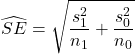
which coincides with the HC2 heteroskedasticity-robust standard error on τ. The default homoskedastic OLS standard error does not, unless the two arms happen to have equal size or equal variance. Exercise 2 puts it to work.
Where a randomised trial can still mislead you
Randomising the offer is not the same as randomising the treatment. If some workers assigned to the course skip it and some controls sneak in, the simple comparison of the groups as assigned estimates the effect of the offer, the intention-to-treat effect. Recovering the effect of actually attending needs the assignment as an instrument. Provided nobody systematically does the opposite of their assignment, and the offer affects raises only through attendance, that identifies a local average treatment effect for compliers; the instrumental variables and 2SLS lesson builds that step.
Attrition is the second trap. If workers who found the course useless quit the firm before raises are recorded, the treated group that remains is no longer a random half. Randomisation protected the start of the trial, not the end. Spillovers are the third: they break SUTVA, and the fix is to randomise whole teams or offices so that the contamination stays inside a unit. Standard errors must then be clustered at that level.
And sometimes you cannot randomise at all. Then the question becomes which assumption replaces the coin flip. Parallel trends, for instance, is the replacement in difference-in-differences.
Three exercises
Exercise 1. Six customers of a bank, with potential outcomes for savings over a quarter in hundreds of USD, are: Y(0) = 10, 8, 6, 4, 3, 2 and Y(1) = 12, 12, 9, 5, 6, 4. The first three chose a budgeting app (D = 1), the rest did not. Compute the ATE, the ATT, the naive gap and the selection bias, and confirm the decomposition.
Answer. The individual effects are 2, 4, 3, 1, 3 and 2, so the ATE is 15/6 = 2.5 and the ATT is (2 + 4 + 3)/3 = 3. The naive gap compares 11, the mean observed Y(1) of the app users, with 3, the mean Y(0) of the rest: 8. Selection bias is the app users’ untreated mean, 8, minus 3, which is 5. Check: 3 + 5 = 8.
Exercise 2. A randomised trial of text-message savings reminders has 100 people in each arm. Mean six-month saving is 52.4 (hundreds of USD) in the treated arm and 47.0 in the control arm, with standard deviations 12 and 10. Estimate the effect, its standard error and a 95% confidence interval.
Answer. The estimate is 52.4 − 47.0 = 5.4. The standard error is the square root of 144/100 + 100/100 = 2.44, about 1.56, giving a t-statistic near 3.46. The 95% interval is 5.4 ± 1.96 × 1.56, roughly 2.34 to 8.46. It excludes zero.
Exercise 3. Return to the eight workers. A lottery puts A, B, E and F on the course. What does the firm estimate, and by how much does it miss the ATE? What is the probability that a lottery reproduces the original self-selected group exactly?
Answer. The treated mean of Y(1) is (9 + 7 + 4 + 4)/4 = 6. The control mean of Y(0), for C, D, G and H, is (5 + 4 + 2 + 1)/4 = 3. The estimate is 3, one thousand above the true 2. That is chance imbalance from the lottery, not bias: the treated four’s untreated raises happen to average 4 against the controls’ 3. Only one of the 70 equally likely draws is {A, B, C, D}, so the probability is 1/70, about 1.4%.
One-on-one with an econometrics tutor in San Diego
Causal-inference courses move fast from this notation to instruments, regression discontinuity and panel designs, and each step assumes you can write the selection-bias decomposition without thinking. If your econometrics sequence at UC San Diego or San Diego State has reached that point, a PhD tutor can take you through your own assignments one question at a time, from the potential-outcomes setup to the standard errors. Book a first session when it suits you.
A first session on causal inference, wherever you study in San Diego
Tell us which course and which problem set, and you will be matched with a PhD tutor in econometrics for one-on-one sessions online. Most students start with the assignment that is due next. The booking form takes a minute, or message us on WhatsApp from the button at the top of the page.
